How to solve a 1D and 2D transient thermal problem in 3D printing technologies like FDM?
- Koohyar Pooladvand

- May 29, 2021
- 8 min read
Updated: Aug 18, 2021
Analytical and computational analyses of FDM processes
Thermal analysis framework
To create a realistic model of the FDM process that includes mechanical and thermal effects, one has to consider solving a highly nonlinear multiphysics problem that faithfully incorporates all influential physics, adequately captures the details of the process, and successfully exemplifies a highly dynamic environment.
Right after the filament leaves the extruder(s), thermal and structural phenomena start affecting the process. The first thermal encounters are radiation and convection on the surface of the filament. The filament also experiences a substantial shear rate inside the nozzle, and when rotates 90 degrees from a vertical to a horizontal direction (see Fig. 1). This shear rate continues to exert force longitudinally when the extruder follows the tool-path as it scans the cross-section. These changes in direction, shears inside the nozzle, and shears during deposition cause the orientation of the added nano- and micro-fiber to be affected significantly. Nozzles used in FDM 3D printers have circular cross-sections; however, the cross-section of the filament when it is laid on the surface or to the contagious filament is semi-ellipsoidal due to the change in direction and pressure. Thus, there are always cavities similar to the one shown in Fig. 1 in the body of the printed components.

Fig. 1. Schematic of the heat transfer model for 1D single-layer deposition of the filament.
Different modes of heat transfer, conduction, convection, and radiation are noticeable in the FDM process. It is also recommended to account for the effect of latent heat around glass transition and softening temperature. Heat dissipation, diffusion, healing, and neck growth affect the material properties of 3D printed components locally in the contact zone. These occurring effects eventually define the structural and geometrical characteristics of a 3D printed component.
Several thermal phenomena are involved in an FDM process. These included convection and radiation with surroundings, conduction with support material and between adjacent filaments, conduction with a heated bed, and radiation and convection in the encapsulated enclosed areas among beads. In addition to those listed in their work, there are several other influential phenomena to consider too, such as changes in conductivity due to temperature, phase change, spatially varying conductivity, thermal resistance between adjacent filament-to -filament, -support material, or -platform, the shape of the filament, and changes in contact areas.
Aside from these factors, there are several other parameters involved known as process and printing parameters such as the position of the component inside the machine, machine environments, air gap, layer thickness, counter thickness, raster angle, orientation, speed, and rate of the deposition.
In addition to process and printing parameters, there are other parameters that relate to manufacturing constraints, for example, fixing mechanism (using vacuum, jig and fixture, or glue), type of the heated bed (metal, glass, or composite), the diameter of the nozzle, stock materials (filament or pellet), type of feeding mechanism, and cooling mechanism.
Each of these parameters has to be considered when the model is developed to make sure the results are reliable and can predict the process correctly.
The computational simulation requires reasonable assumptions. Some of the critical and widely accepted assumptions, have appeared in several proposed numerical approaches, are listed hereunder:
material is deposited discontinuously at each time step,
The process, in reality, is continuous, but for modeling the deposition is assumed to take place sequentially at time step; thus, the volume of the deposited material will be equal to the feed rate multiplied by this time step,
material leaves the extruder in equilibrium thermal condition with its temperature equals to extruder temperature. If the nozzle is large and heating is unstable, this assumption is not valid, and experimental measurement is required to find the relationship between the set temperature and the leaving temperature,
the relevant boundary conditions are updated as the part proceeds according to the latest local circumstances,
material properties are updated as the simulation continues based on local conditions,
enthalpy formulation is used to model the effects of phase changes.
In an attempt to produce a reliable simulation, this dissertation incorporated assumptions mentioned above and applied other considerations explained in the following section.
The general scheme of the thermal model
Radiation, advection, and convection are the three primary sources of heat loss on the boundaries of the thermal domains. Radiation has been ignored in several studies of FDM, arguing its effect is not comparable to the convection and conduction heat transfer. Although the effect of radiation for small diameters is negligible compared to the effect of convection, in large diameters, it must be included in the model.
Convection is a significant source of heat loss, and its dependency on temperature and size pertains to accurate thermal flow estimation. However, in several studies, the constant value of the coefficient of heat convection, hcov, was used, one can incorporate the experimental correlation for this thermal coefficient.
Governing equations
Conservation of mass, momentum, and energy define the framework of the governing equations; however, it also required to contemplate hydrodynamics and rheology of materials to encompass the thermo-fluid-mechanical effects accurately. The first set of equations is the conservation of mass:

where V is velocity, ρ is density, and subscripts x, y, and z refer to three axes in the Cartesian system r, θ, and z are three directions in the cylindrical coordinate. Equation (2) defines the general form of the conservation of energy:

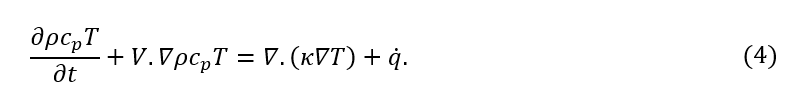
where E is energy, W work, and CV control volume. Equation (3) is used to develop the governing equation for transient heat transfer with phase transition and enthalpy formulation.

where t is time, u internal energy, ρ mass density, V velocity vector, h enthalpy, conductivity, T temperature, and q the volumetric heat generation.

Fig. 2. 3D elements and schematic representing a 2D cylindrical fabrication model with symmetry in direction: (a) cylindrical element at node i, j; (b) first radial ring is being deposited from perimeter toward center; (c) last radial ring is being deposited on the same layer at the center, and (d) first radial ring is being deposited on the next layer.
Furthermore, by realizing du=dh=cp.dT, and cp is specific heat capacity, the governing equation (3) reads as:
The thermal problem, in general, is complex and 3-dimensional and requires high-performance computing (HPC) to capture a transient thermal problem with high fidelity.
It is possible to simplify the 3D problem to 2D without sacrificing the governing physics. For example, the governing equation can be analyzed with symmetry about the θ axis in a cylindrical coordinate for a cylinder manufactured in z-direction continuously, as shown in Fig. 2. In such a 3D problem, we used the following PDE derived from Eq. (4) to solve for temperature distributions:

The 1D model analytical framework
A simplified 1-D model to analyze heat transfer in FDM is achievable. This model was developed by assuming a lumped-capacity criterion. This assumption was made because the heat convection coefficient was large enough in the presence of a small diameter (e.g., 500μ) and low conductivity (e.g., 0.17 W/mK) to lower the Biot number to less than 0.1. Such a low Biot number suggests the temperature distribution along the cross-section is uniform and relaxes the demand for a 2D and 3D simulation. In such a model, the temperature of the hot-end, heated-bed, and the environment was assumed constant, and the extruder moved with a fixed velocity equal to U. For this problem, the partial differential equation can be obtained as described here and illustrated in the following:

here q with different subscripts indicates heat fluxes, with con, conv, neight, and rad being conduction, convection, neighbor, and radiation, respectively. Ac is the cross-sectional area, Ah is the perimeter area for convection and radiation, Ai is the contact area to bed or another filament, ε is the emissivity, and σ is the Stefan-Boltzmann constant. Also, T and T∞ are the surface and environment-wall temperatures. is heat transfer coefficients, and subscripts i indicates the different neighbors, i.e., heated-bed or other filaments. The filament can be placed on the bed or the previously deposited material; thus, is either heated bed temperature or the corresponding temperature of the surrounding filament.
A simplified condition can be assumed as a semi-infinite case of continuous filament depositing on the heated bed. One can assume a large heat convection coefficient for air and large volume for bed, introduce a total hT, and neglect the effect of the deposited filament on a heated bed. Figure 1 illustrates the assumed condition. Finally, Eq. (4) can be simplified to:
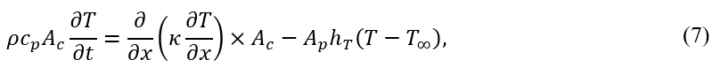
where, Ac and Ap are cross-section and perimeter of the filament, respectively.
Knowing that,
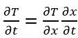
, and assuming the constant velocity for hot-end equal to,

Eq. (7) can be rewritten as:
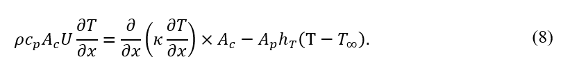
hT is defined as a total convection-contact-radiation heat transfer coefficient. In other words, the heat transfer due to the contact to the heated bed was also added to convection and radiation:

reff is the ratio of the heated bed contact area of the filament perimeter. The Eq. (9) can be solved analytically as follow:

with
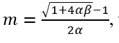
where,

and T_ext is extruder temperature.
1D modeling of a slender cylinder satisfies lumped-capacity criterion
The 1D model for studying the case can be extended to a cylindrical part manufactured in a 3D printer. This case was analogous to filament deposition, but the whole cross-section of the cylinder was assumed to be laid continually with a known temperature at a selected time increment commensurate with the layer thickness. It means we assumed that the whole cross-section was deposited with the velocity equal to the deposition velocity of the whole layer. The developed 1D model is illustrated in Fig. 3-a.

Fig. 3. Schematics of the proposed 1D model for numerical analyses: (a) The addition material simplification as an advent deposition of the whole layer with the velocity of U at time increment dt=dL/U; and (b)representative schematic of energy balance for a 1D model in a cylindrical coordinate system for deposition of the i-th layer.
In order to ensure the lumped-capacity criterion was still valid, the diameter had to be chosen to satisfy the Biot number less than 0.1 knowing martial properties (conductivity and density) and environmental constraints (specifically coefficient of convection heat transfer).
Energy balance for such a cylindrical specimen with depicted boundary conditions in Fig. 3-b is obtained as:

where all the parameters are defined before. By substituting Eqs (10-b) and (10-c) into Eq. (10-a), we reached:
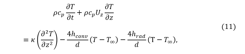
where T and T∞ are surface and environment-wall temperatures, respectively, d is the diameter, and hrad is the radiation heat transfer coefficient:
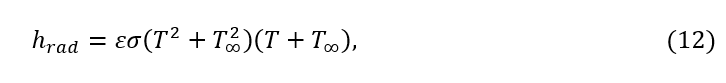
This radiation heat transfer coefficient was added to the convection heat transfer, h_conv, to define the total heat transfer coefficient, ht, as follows

Determination of ht values is crucial for accurate simulations. This total heat transfer coefficient was approximated empirically by exponential functions as:

where α and β are determined by experimental investigations and procedures. We also estimated ht for FDM by combining radiation and convection heat transfer through a combined experimental-computational approximation using a 1D model.
A 2D model analytical framework
The physics in FDM deposition is complex, and adding the nonlinearity of the material properties and boundary conditions to the problem makes the analytical solution hardly possible. However, one can solve analytically by applying several simplifications, such as a rectangular cross-section, seamless contact between layers, constant heat transfer coefficient, constant material properties, and deposited material temperature equal to the extruder temperature. In a vertical stacking assumed in x-direction, one can reach the following analytical solution:
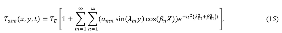
where,

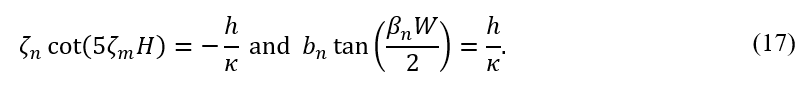
where T_ave, is averaged temperature between the envelope temperature, T∞, and the liquefier temperature, Text. H and W are the filament’s height and width. The eigenvalues are the roots of the following transcendental equations:
References:
[1] Pooladvand, K., 2019, "Multifunctional Testing Artifacts for Evaluation of 3d Printed Components by Fused Deposition Modeling," Worcester Polytechnic Institute, [Link].

Comments