1D transient thermal in AM, how to write a code in MATLAB(R) to solve the PDE for Fourier's law?
- Koohyar Pooladvand

- Jul 5, 2021
- 8 min read
Updated: Aug 18, 2021
The complexity of layer-by-layer modeling of AM is evident in the consolidation of many thermo-mechanical cycles. Inevitable present of residual stress due to cyclic thermomechanical events, phase change and high spatial and temporal gradient of temperature, besides the part geometry, AM process parameters and mechanical and environmental parameters form the product final shape. The whole body at various levels will meet the cycle of melting, solidification, phase change and heat flux that not only change the mechanical properties, but also have effect on final product quality, shape, and microstructure.
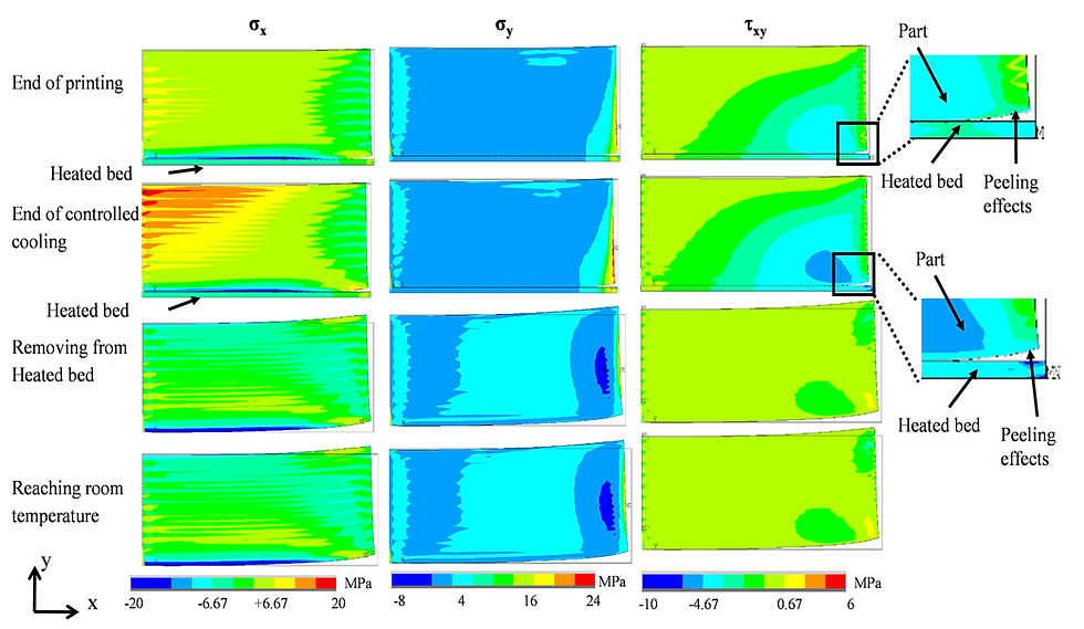
Figure 1: Stress development in additive manufactured parts due to heat cycle.
The process of formation and production of a part by additive manufacturing involves all sources of heat transfer: convention, conduction, and radiation. Radiation plays a particularly important role in the first phase of material composition. The development of residual stresses in part depends on the way the parts cool until conduction and convection comes to a more vital role in lower temperature and converts the case to a sophisticated problem, where all kinds of heat transfers must be taken into account. Since radiation comes to play a crucial role, it brings nonlinearity to the problem and solving the boundary condition problem will be more complicated.
One can model a simple additive manufactured part, by applying simplification to the multiphysics problem and condensing it down to a simpler problem by only considering the effect of heat transfer. One may try to find the AM process parameters effect to make the final product more reliable with less undesired deformed shape and internal residual stresses. In this study, instead of 3D or 2D computational modeling, one dimensional case like a cylinder with thin diameters made by 3D printer is studied, the material is ABS and because of the deposition case the laser beam is not applicable. So the problem is simplified but still all sources of heat transfer are considered and the nonlinearity because of transient modeling, radiation heat transfer in the boundary and mass transfer cause enough hurdle to make modeling challenging and case close to real situation.

Figure 2: Scheme of Layer-by-Layer deposition of cylindrical part
Problem Formulation and Numerical Method:
The total energy transferred is absorbed by the volume of material in contact with, where the absorbed energy will be transferred by heat conduction further into the interior of the target or caused phase change or evaporation if the energy is large enough. In this case, one studies the 3D printer in which the material deposition layer-by-layer takes place to form the part.
The mathematical and physical underlying modeling of part formation is rooted in conservation of mass, momentum, and energy equation by considering the phase change and property changes of material.
To model the transient heat transfer with phase transitions, researcher proposed enthalpy formulation. The general equation of convection-diffusion is:

Where, u is internal energy, h the enthalpy, ρ the density, k the conductivity, q dot is volumetric heat source. T the temperature and V the speed of either the heat source or the medium. In most applications, the origin of the coordinate system is fixed to the center of the heat source on top of the processed surface. x is the direction of heat source, y perpendicular to that in the plane and z the normal to the plane or motion.
Figure 2 illustrates our case where the z direction is chosen in the assembly direction where the deposition is taking place in constant velocity equal to U. The first equation to be satisfied is the mass conservation that is written and simplified as:
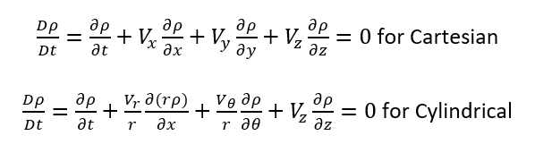
Where Vx, Vy, Vr, and Vθ are 0 and Vz=U, then for both coordinates:

The next main equation is the energy conservation, knowing that du=dh=Cp*dT for solid and liquid. The governing equation is Fourier’s law of heat convection and for 2D cylinder this equation could be written in the following format where z is the deposition axis and r is the radius direction and because of symmetry the Ө is not considered.

And by simplification, as Vx, Vy, Vr, and Vθ are 0 and Vz=U and the symmetry in Ө direction, we get to:

Where t is time, z is axial coordinate, r radial coordinate, T temperature, and k the thermal conductivity coefficient.
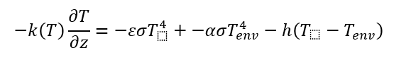
For boundary condition on the surface in contact with heat flux (energy flux I(t) ) and for other the heat loss is taken into account.

Where, α is the absorbance, ε the emissivity and σ the Stefan-Boltzmann constant. And Ts, T∞ and TExt are the surface, environment-wall and extruder temperature receptively. One assumes that the ambient temperature if the chamber is either filled by inert gas or air is equal to chamber wall temperature. The chamber medium is not participating and the absorptivity is 0. In most cases, since the order of convection and heat dissipation flux are not in the order of incident heat, the boundary condition is simplified to:

If the vaporization or mass flow are taken place two more boundary conditions should be added:

Where U in the mass deposition velocity and Uv and Lv is Vaporization rate and vaporization latent heat respectively. In our case ε=1 and we can assume Ts = T∞, additionally the laser heat incident is zero and the phase change is not considered so:

But one further action could be taken instead of modeling the 2D, by assuming lump condition that Biot number is less than 0.1 (the radius of the cylinder is small), so the 2D heat distribution could be simply boiled down to one dimension. In this case our differential element is cylinder in z direction with the differentia length equal to dz (Figure 4).

Figure 4: Cylindrical Element

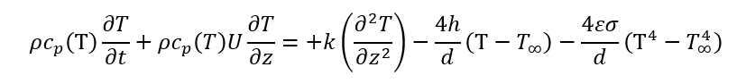
Where A is equal to, A = Pi*r^2 , then:
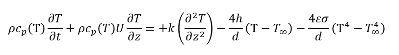
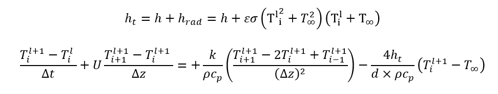
For avoiding the nonlinearity because of the power of 4 in radiation, this term will be considered as convection heat transfer coefficient where the hrad is:
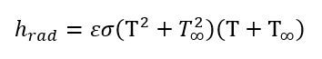
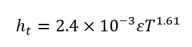
Frewin and Scott proposed a simple model for ht to consider the convection and radiation in the same time. This recommended correlation is chosen to be used instead aforesaid ht to make the calculation simple and straight forward.
To solve the set of equations we need two more conditions, which one would be the initial value at the time equal to 0, and another is the boundary condition at the other end. In our case, the very thin layer of material in considered place on the base surface which is in equilibrium with the basement that is kept in a fixed temperature (Tbase=70 oC). As the base temperature is fixed it satisfies our next boundary condition as well.

Finite Difference Model:
To solve the governing equation, the finite difference scheme is utilized. The basic steps in obtaining a numerical solution using finite difference are categorized as follows [11, 17].
1. State the mathematical statement of the problem in terms of governing equations, boundary conditions and initial conditions.
Discretize the solution domain into a network of discrete nodal points. The unknown values are sought only at those discrete points rather than obtaining a continuous solution in the domain.
Obtain discretization equations for all nodal points by approximating the governing differential equations and boundary conditions. This discretization procedure leads to a set of algebraic equations involving the unknown values at the nodal points.
Use an appropriate solution algorithm to solve the set of algebraic equations involving the unknown values at the nodal points.
Post-processing of the data to evaluate secondary quantities.
To solve the governing equations the finite difference scheme is utilized, implicit Euler is used for time integration:
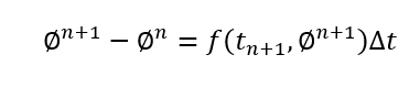
Where ϕ = T in our case.
For the convective term, a first order upwind difference scheme is used. For V>0, this becomes:
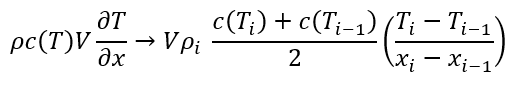
And for diffusive terms:
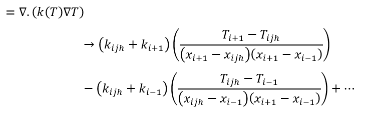
The material parameters are evaluated at moment t, for each time step, the equation can be written as:

To solve the boundary condition, the real situation of our case is taken into account where the bottom which is placed in the 3D printer is heated by a plate that keeps the temperature equal to Tbottom=70 oC, the top is the location of the heat source which should be modeled carefully, and the sides are the radiative and convection to the ambient temperature:

At vertical boundary as a cylinder, because of symmetry we can assume that:
Discussion:
The material properties of the ABS are described hereunder in the appendices section where the main characteristics such as the mass density (ρ), conductivity (κ), and specific heat (Cp) were taken to be 1.04 g/cm3, 0.17 W/m-K, and 1400 J/kg-K respectively. In order to validate the code and finite differential equation set up. I compared the solution of semi-infinite problem with the code outcome. The solution related parameters are noted in table 1.

The solution of semi-infinite case is available which is:

Where erfc is complimentary error function, and α is diffusivity (α=k/ρ Cp = .117 x 10^-7 ), additionally in this case, T1 is the T platform. In modeling this comparison the Deposition velocity and the extruder temperature are put to zero and the convection coefficient as well. The part is considered in its full length by putting the Z0 equal to the desired part length (L=50mm) at start point.

Figure 5: Comparison of temperature for 2 different node @ 3 and 5 mm from base between analytical and numerical solution
Figure 5 and 6 depict the temperature of analytical and numerical solution for 2 different nodes in the part and all points over about 20 minutes respectively. One can admit the results are matched well and the numerical solution is validated for 1-D Finite Difference solution in our case.

Figure 6: Temperature distribution along part Vs. time
The input parameters of the Figure 7 and 8 are listed in table 1. These two figures illustrate the temperature in the node in contact with extruder and the temperature in part during cooling.

Figure 7: Temperature over time at the first node in contact with extruder
The temperature of the top point increased by time to reach to the maximum and will be constant until the part is completed, and the cooling will start later when this temperature gets cooler until reach to ambient temperature finally.
Figure 8 depicts the temperature distribution along the part during cooling phase and as someone can expect the exposed point to the top will confront with maximum heat flux and the maximum temperature takes place in some where beneath the exposed node and the part temperature reaches lower and lower till be equal to ambient temperature.

Figure 8: Temperature along part during cooling
TIME DISCRETIZATION PROCEDURE IMPLICITLY:
Because of the physics of our case and the progression of z elements in time, explicit scheme does not work well and one must do the implicit scheme to find the result in each step. So the following illustrate the implicit configuration and the theory and the constant development.
The related. Differential equations to be solved is:
If we use the explicit scheme for time and location, we will obtain the following

Where ht is:
And then:


As you can see in this case, the temperature in each node in this step is unknown and the related system of linear equation should be solved for each step to give us the results. To complete the system of equation we still need two more equations that we are going to have by applying the boundary condition.
Thus, at the one end, Lt the temperature is fixed.

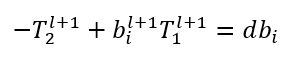
At another end we have:

And,

The next step would be the numerical modeling of it when the length reaches the desired length and let it be cooled until room temperature.
Where,

And finally, at time equal to 0, the layer of material with the thickness of 0.3 mm is already laid on the table which its temperature is 343.15 K.
So, by starting from t=0 and marching in time and finding the system of equations constant we will have the temperature in each node. One more things worth to mention is that the implicit solution is not as sensitive as explicit solution to convergence criteria which will allow us to choose the spatial step equal to:

And then the fluctuation because of this inequality will not be a problem anymore and the results are smoothly achieved.
Code Flow Chart for explicit scheme:

References:
[1] Pooladvand, K., 2019, "Multifunctional Testing Artifacts for Evaluation of 3d Printed Components by Fused Deposition Modeling," Worcester Polytechnic Institute, [Link].

Comments